PID Loop Simulator
The PID Loop Simulator is an Excel tool to simulate a Proportional, Integral and Derivative (PID) controller on a First Order Time Delay (FOTPD) process. Both open and closed loop processes can be simulated using this powerful tool. This is a great tool for learning the basics of PID control and loop tuning.
Download
PID_Loop_Simulator.xlsxHow to use
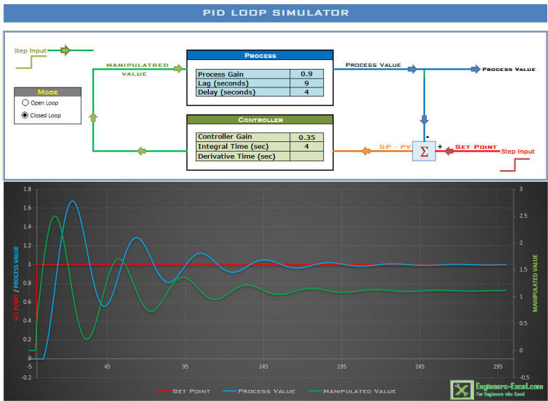
The First Order Time Delay (FOTPD) process has 3 parameters – Process Gain, Lag Time and Delay Time. (Details of these parameters are given in the "Process Model" section below.) These parameters should be entered under the “Process” section of the Simulator.
Enter the controller values in the "Controller" section. These parameters are the controller gain, integral time in seconds and the derivative time in seconds.
Choose the “Open Loop” option to view the open loop response. In this mode, the controller is not used. The chart shows the effect of a step change in the manipulated variable (such as a control valve) on the process value.
The tool simulates the parallel form of the PID equation, this is form that is widely used in academic environments
. The equation implemented is:
where:
t = Time
MV = Manipulated Value
K = Controller Gain
e = Controller error = Set Point - Process Value
T i = Integral Time
T d = Derivative Time
Feedback and Contributions from Visitors
The PID Simulator tool has been the most downloaded tool on this site and I am grateful to the users who sent me a lot of positive feedback about it.
Torcuato Fernandez pointed out an error in original version, which has since has been corrected. I would like to thank Torcuato for pointing out the error.
I would also like to thank Hannu Lehmuskuja for pointing out an error related to the delay.
Jose Maria, has shared some of his work with me and has kindly agreed to let me share it with others through this site. He has added scrollbars to the tool, which assist the user understand how the controller settings affect the loop.
Download the file here.
Thanks to William Poetra Yoga who has ported this tool to Google Sheets. The file can be accessed here. William has also kindly provided a link to these instrunctions for users who may want to copy the file to their account and modify it.
PID Loop Simulation and Tuning tool for the Industry
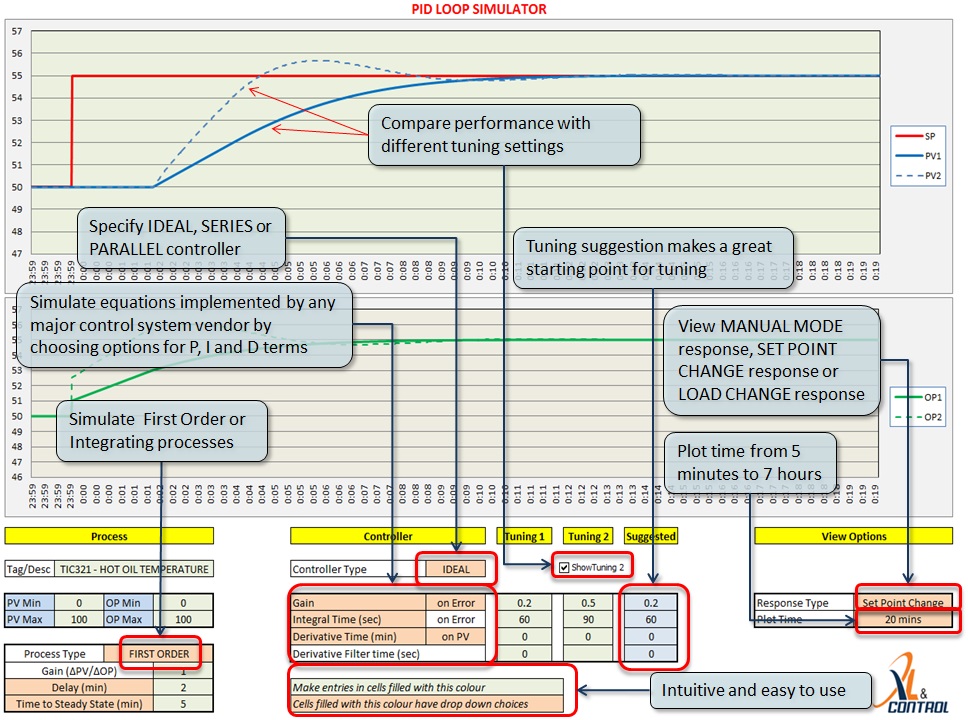
The use of PID Controllers is widespread in the process industry. Industrial controllers use different forms of the PID controllers. A powerful PID simulation tool that can simulate these different forms and be used for loop tuning is available at the business site www.xlncontrol.com. Features of this tool are shown below. (A free demo version is also available with limited features.)
Process Model
To use the simulator, we need a model of the process. Obtaining the process parameters is known as System Identification.
Most chemical processes fall into one of 2 categories - first order process with dead time (FOPDT) and integrating processes with dead time. This app works with the former.
An FOPDT process is characterised by 3 parameters:
1. Process Gain - the ratio of the change in process variable to the ratio of the change in manipulated variable
2. Time constant - which measures the speed of response
3. Dead time - time between moving the manipulated variable and start of the process response
One of the most common ways of obtaining these parameters is by doing a step test. To do this, wait for the process to be steady and then step the Manipulated Variable (MV). The process variable (PV) will move as shown below.
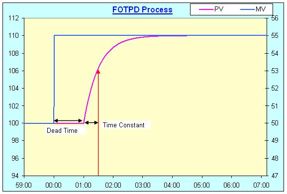
Calculate the parameters as follows:
Dimensionless Gain = (Change in PV/PV range)/(Change in MV/MV Range)
Time constant = Time taken for the PV to change by 63.2% of the final change
Dead time = Time for the PV to start moving after the change in the MV
For the step response shown in the figure above, Dimensionless Gain = (10/200)/(5/100), where PV range = 200 units and MV range = 100 units
Time constant = 30 sec
Dead time = 60 sec
Key in these parameters into the simulator and study the effects of changing the tuning parameters on the response of the system.
Why 63.2% ?
The response of a delay free first order system is described by:
Change in PV = Process gain x (1 - exp(-Time/Time Constant))x Change in MV
Since the final change in PV = Process gain x Change in MV, this equation can be written as
Change in PV = Final Change in PV x (1 - exp(-Time/Time Constant))
At time = time constant,
Change in PV = (1 - exp(-1)) x Final Change in PV = 0.632 x Final Change in PV or 63.2% of the final change in the PV
I would like to thank Hannu Lehmuskuja to correcting an error in these equations.
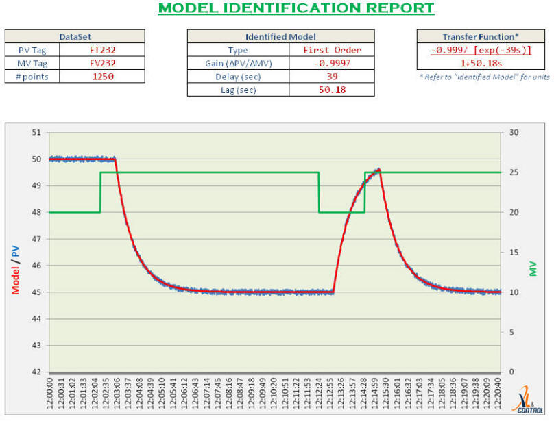
System Idenfitication Tool
In the industrial environment, it is often difficult to obtain process models due to noisy data. A powerful for system identfication is available at the business site www.xlncontrol.com
How it works
There are 2 worksheets in the Excel file, the calculations required for the simulation are done on the sheet "PID Calculations".
Defined Formulae are used in the computation.
The first order process is calculated using a difference equation, given by:
Process Value = b x (Output at time offset by delay time) - a x Last PV; where
a = - exp ( -1 / Process Time Constant) and
b = Process Gain x (1 + a)
The error is calculated by taking the difference between the PV and SP values. The error values are accumulated in column F for the integral term calculation and the derivative term is calculated by taking the difference between the current error and the last error. The PID calculation determines the next output value. The PID calculation is:
The next output value is calculated using:
Controller Gain x error + Accumulated error / Integral time + Derivative x (Current error - Previous error)
The calculations are repeated at every second to obtain the response, which is plotted on the chart on the first sheet.